Background

Risk Navigator (SM) has two Adjusted Vega columns that you can add to your report pages via menu Metrics → Position Risk...: "Adjusted Vega" and "Vega x T^-1/2". A common question is what is our in-house time function that is used in the Adjusted Vega column and what is the aim of these columns. VR(T) is also generally used in our Stress Test or in the Risk Navigator custom scenario calculation of volatility index options (i.e VIX).

Abstract

Implied volatilities of two different options on the same underlying can change independently of each other. Most of the time the changes will have the same sign but not necessarily the same magnitude. In order to realistically aggregate volatility risk across multiple options into a single number, we need an assumption about relationship between implied volatility changes. In Risk Navigator, we always assume that within a single maturity, all implied volatility changes have the same sign and magnitude (i.e. a parallel shift of volatility curve). Across expiration dates, however, it is empirically known that short term volatility exhibits a higher variability than long term volatility, so the parallel shift is a poor assumption. This document outlines our approach based on volatility returns function (VR(T)). We also describe an alternative method developed to accommodate different requests.

VR(T) time decay

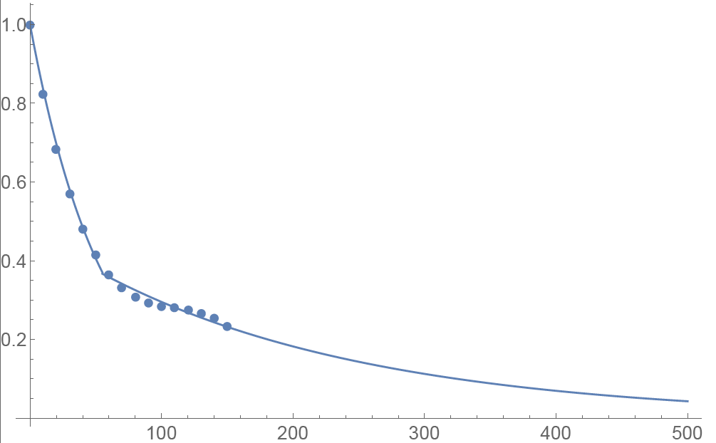
We applied the principal component analysis to study daily percentage changes of volatility as a function of time to maturity. In that study we found that the primary eigen-mode explains approximately 90% of the variance of the system (with second and third components explaining most of the remaining variance being the slope change and twist). The largest amplitude of change for the primary eigenvector occurs at very short maturities, and the amplitude monotonically decreases as time to expiration increase. The following graph shows the main eigenvector as a function of time (measured in calendar days). To smooth the numerically obtained curve, we parameterize it as a piecewise exponential function.

Functional Form: Amplitude vs. Calendar Days

To prevent the parametric function from becoming vanishingly small at long maturities, we apply a floor to the longer term exponential so the final implementation of this function is:

where bS=0.0180611, a=0.365678, bL=0.00482976, and ^T*=55.7 are obtained by fitting the main eigenvector to the parametric formula.

Inverse square root time decay

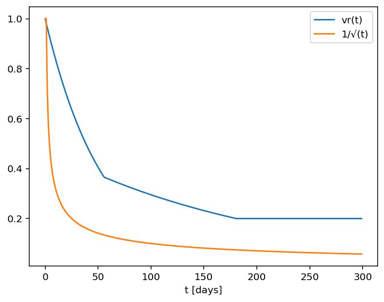
Another common approach to standardize volatility moves across maturities uses the factor 1/√T. As shown in the graph below, our house VR(T) function has a bigger volatility changes than this simplified model.

Time function comparison: Amplitude vs. Calendar Days

Adjusted Vega columns

Risk Navigator (SM) reports a computed Vega for each position; by convention, this is the p/l change per 1% increase in the volatility used for pricing.  Aggregating these Vega values thus provides the portfolio p/l change for a 1% across-the-board increase in all volatilities – a parallel shift of volatility.

However, as described above a change in market volatilities might not take the form of a parallel shift.  Empirically, we observe that the implied volatility of short-dated options tends to fluctuate more than that of longer-dated options.  This differing sensitivity is similar to the "beta" parameter of the Capital Asset Pricing Model.  We refer to this effect as term structure of volatility response.

By multiplying the Vega of an option position with an expiry-dependent quantity, we can compute a term-adjusted Vega intended to allow more accurate comparison of volatility exposures across expiries. Naturally the hoped-for increase in accuracy can only come about if the adjustment we choose turns out to accurately model the change in market implied volatility.

We offer two parametrized functions of expiry which can be used to compute this Vega adjustment to better represent the volatility sensitivity characteristics of the options as a function of time to maturity. Note that these are also referred as 'time weighted' or 'normalized' Vega.

Adjusted Vega

A column titled "Vega Adjusted" multiplies the Vega by our in-house VR(T) term structure function. This is available any option that is not a derivative of a Volatility Product ETP. Examples are SPX, IBM, VIX but not VXX.

Vega x T^-1/2

A column for the same set of products as above titled "Vega x T^-1/2" multiplies the Vega by the inverse square root of T (i.e. 1/√T) where T is the number of calendar days to expiry.

Aggregations

Cross over underlying aggregations are calculated in the usual fashion given the new values. Based on the selected Vega aggregation method we support None, Straight Add (SA) and Same Percentage Move (SPM). In SPM mode we summarize individual Vega values multiplied by implied volatility. All aggregation methods convert the values into the base currency of the portfolio.

Custom scenario calculation of volatility index options

Implied Volatility Indices are indexes that are computed real-time basis throughout each trading day just as a regular equity index, but they are measuring volatility and not price. Among the most important ones is CBOE's Marker Volatility Index (VIX). It measures the market's expectation of 30-day volatility implied by S&P 500 Index (SPX) option prices. The calculation estimates expected volatility by averaging the weighted prices of SPX puts and calls over a wide range of strike prices.

The pricing for volatility index options have some differences from the pricing for equity and stock index options. The underlying for such options is the expected, or forward, value of the index at expiration, rather than the current, or "spot" index value. Volatility index option prices should reflect the forward value of the volatility index (which is typically not as volatile as the spot index). Forward prices of option volatility exhibit a "term structure", meaning that the prices of options expiring on different dates may imply different, albeit related, volatility estimates.

For volatility index options like VIX the custom scenario editor of Risk Navigator offers custom adjustment of the VIX spot price and it estimates the scenario forward prices based on the current forward and VR(T) adjusted shock of the scenario adjusted index on the following way.

• Let S0 be the current spot index price, and
• S1 be the adjusted scenario index price.
• If F0 is the current real time forward price for the given option expiry, then
• F1 scenario forward price is F1 = F0 + (S1 - S0) x VR(T), where T is the number of calendar days to expiry.

A combination order is a special type of order that is constructed of multiple separate positions, or ‘legs’, but executed as a single transaction.  The legs of the combination may be comprised of the same position type (e.g. stock vs. stock, option vs. option or SSF vs. SSF) or different position types (e.g. stock vs. option, SSF vs. option or EFP).  It’s important to note that many combination order types, while submitted via the IB trading platform as a combination, are not native to (i.e., supported by) the exchanges and therefore may not be guaranteed by IB.  Accordingly, IB’s policy is to guarantee only Smart-Routed U.S. stock vs. option and option vs. option combination orders.

As combination orders which are not guaranteed are exposed to the risk of partial execution, both in terms of the quantity of legs and their balance, IB requires account holders to acknowledge the 'Non-Guaranteed' attribute at the point of order entry.  There are two methods for setting this attribute:

• Method 1 - Users can select the Non-Guaranteed attribute in the Misc. section on the Order Ticket for a particular order
• Method 2 - Users can add the Non-Guaranteed column to the Order Management section of the TWS

Notes:

• Non-Guaranteed combination orders are not available for Financial Advisor allocation orders

The risk of such 'Non-Guaranteed' orders is illustrated through the example below:

Example

Assume the following quotes for a Stock vs. Stock combination order to purchase shares of Microsoft (MSFT) and sell shares of Appl (AAPL).

Current markets

MSFT - 26.30 bid, 26.31 offer
AAPL - 250.25 bid, 250.30 offer

A generic combination is created to buy 1 share AAPL and sell 1 share MSFT, the implied quote would be 223.94 bid, 224 offer.

The following order is entered:
Buy 200 AAPL, Sell 200 MSFT
Pay 224

Based on the current markets, the order would appear to be executable.

• A buy of 200 shares of AAPL are routed with a 250.30 limit. Only 100 execute.
• A sell of 200 shares of MSFT are routed with a 26.30 limit. No execution is received as the market moves to 26.29 bid.

With a Non-Guaranteed combination, the 100 shares of AAPL would be placed in the client account, even though no MSFT shares were executed.  The remainder of the combination order will continue to work until executed in its entirety or until it is canceled.

How to create option spread strategies using OptionTrader